1.C++相关
(1)继承
单继承的定义格式如下
class <派生类名>:<继承方式><基类名>
{
	<派生类新定义成员>
};
<继承方式>常使用如下三种关键字给予表示:
- public 表示公有基类;
- private 表示私有基类;
- protected 表示保护基类;
(2)Eigen库数据结构内存对齐
在自定义的类中,如果成员中有Eigen的数据结构,可能会出现内存不对齐的问题。
class Foo
{
  //...
  Eigen::Vector2d v;
  //...
};
//...
Foo *foo = new Foo();
在使用这个类的时候用到了new方法,这个方法是开辟一个内存,但是在上面的代码中没有自定义构造函数,所以在new的时候会调用默认的构造函数,调用默认的构造函数的错误在于内存的位数不对齐,所以会导致程序运行的时候出错。解决的方法就是在类中加入宏EIGEN_MAKE_ALIGNED_OPERATOR_NEW。
 class Foo
{
  ...
  Eigen::Vector2d v;
  ...
public:
  EIGEN_MAKE_ALIGNED_OPERATOR_NEW
};
(3)C++模板类
之前介绍了C++中的模板函数,但其实模板类也是类似的。和之前相同,模板参数列表里可以有不止一个参数。例如下面就是一个例子:
/**
 * \brief Templatized BaseVertex
 *
 * Templatized BaseVertex
 * D  : minimal dimension of the vertex, e.g., 3 for rotation in 3D
 * T  : internal type to represent the estimate, e.g., Quaternion for rotation in 3D
 */
  template <int D, typename T>
  class BaseVertex : public OptimizableGraph::Vertex {
  	//...
  }

class CurveFittingVertex: public g2o::BaseVertex<4, Eigen::Vector4d>{
	//...
}
(4)虚函数
在基类用virtual声明成员函数为虚函数。这样就可以在派生类中重新定义此函数,为它赋予新的功能,并能方便被调用。
在派生类中重新定义此函数,要求函数名,函数类型,函数参数个数和类型全部与基类的虚函数相同,并根据派生类的需要重新定义函数体。c++规定,当一个成员函数被声明为虚函数后,其派生类的同名函数都自动成为虚函数。因此在派生类重新声明该虚函数时,可以加virtual,也可以不加,但习惯上一般在每层声明该函数时都加上virtual,使程序更加清晰。如果再派生类中没有对基类的虚函数重新定义,则派生类简单的继承起基类的虚函数。
基类中若虚函数=0,则在派生类中必须要重新定义该虚函数,例如下面这几个函数都是基类中的虚函数,且需要在派生类中重新定义。
        /**
         * update the position of the node from the parameters in v.
         * Implement in your class!
         */
        virtual void oplusImpl(const number_t* v) = 0;

        //! sets the node to the origin (used in the multilevel stuff)
        virtual void setToOriginImpl() = 0;
        //! read the vertex from a stream, i.e., the internal state of the vertex
        virtual bool read(std::istream& is) = 0;
        //! write the vertex to a stream
        virtual bool write(std::ostream& os) const = 0;
(5)static_cast关键字
用法
static_cast <type-id> (expression)
static_cast叫做编译时类型检查。该运算符把expression转换为type-id类型,这样做的目的是在程序还没有运行时进行类型检查,来保证转换的安全性。
而与之对应的,dynamic_cast关键字(运行时类型检查)主要用于类层次结构中父类和子类之间指针和引用的转换,由于具有运行时类型检查,因此可以保证下行转换的安全性。即转换成功就返回转换后的正确类型指针,如果转换失败,则返回NULL。
所谓上行转换是指由子类指针到父类指针的转换,下行转换是指由父类指针到子类指针的转换。
(6)Eigen中的数据类型
在Eigen中已经定义好了很多与旋转、变换等有关的数据类型,我们直接使用就可以了,不需要再重新定义了。
- 旋转矩阵(3 3):Eigen::Matrix3d
- 旋转向量(3 1):Eigen::AngleAxisd
- 欧拉角(3 1):Eigen::Vector3d
- 四元数(4 1 ):Eigen::Quaterniond
- 欧式变换矩阵(4 4):Eigen::Isometry3d
- 仿射变换矩阵(4 4):Eigen::Affine3d
- 射影变换矩阵(4 4):Eigen::Projective3d
(7)SIZE_T
它可以用来表示非常大的数字范围,可以充分利用计算机的位数,比int、long等范围更大。
(8)循环
for(auto e:edges){
    //code...
  }
C++中for循环的简略写法,类似Python中的循环写法。
2.g2o库简介与编译安装
g2o全名叫General Graph Optimization,通用图优化。由字面意思即可理解,即只要是一个优化问题能转成图优化的形式就可以使用g2o来解决。
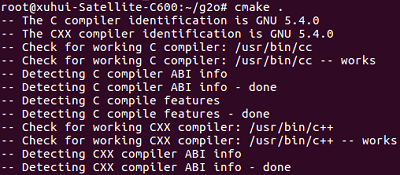
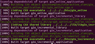
首先从g2o的Github网页上下载源码,解压。然后cd到解压目录下,如果不想麻烦,直接cmake .,然后make,最后make install即可大功告成。g2o编译依赖于Cmake和Eigen两个库,这两个库都非常好安装,如果没有安装,百度一下如何安装就可以了。
3.图优化曲线拟合
将曲线拟合问题抽象成图优化,只需要记住节点为优化变量,边为误差项。
在曲线拟合问题中,整个问题只有一个顶点:曲线模型参数,而各个带噪声的数据点,构成了一个个误差项,也即图优化的边。但这里的边是一元边(Unary Edge),即只连接一个顶点。因为整个图只有一个顶点,所以只能画成自己连接到自己的样子。在图优化问题中,一条边可以连接一个、两个或多个顶点,这反映了每个误差与多少个优化变量有关。这种边也叫做超边(Hyper Edge),整个图叫超图(Hyper Graph)。
4.图优化曲线拟合实例
下面针对一个具体的问题来实际练习g2o的使用,拟合函数
\[y = exp(3.5x^3+1.6x^2+0.3x+7.8)\]整个图优化的流程如下:
- (1)定义顶点和边的类型
- (2)构建图
- (3)旋转优化算法
- (4)调用g2o优化,返回结果
首先新建一个项目,然后在CMakeLists文件里引用g2o和相关库。
cmake_minimum_required(VERSION 2.6)
project(g2o_test)

set( CMAKE_CXX_FLAGS "-std=c++11 -O3" )

# 添加cmake模块以使用ceres库
list( APPEND CMAKE_MODULE_PATH ${PROJECT_SOURCE_DIR}/cmake_modules )

# 寻找G2O
include_directories(
    ${G2O_INCLUDE_DIRS}
    "/usr/include/eigen3"
    "/usr/include/suitesparse"
)

# OpenCV
find_package( OpenCV REQUIRED )
include_directories( ${OpenCV_DIRS} )

add_executable(g2o_test main.cpp)

# 与G2O和OpenCV链接
target_link_libraries( g2o_test
    ${OpenCV_LIBS}
    g2o_core g2o_stuff
)

install(TARGETS g2o_test RUNTIME DESTINATION bin)
然后编写代码文件。
#include <iostream>
#include <g2o/core/base_vertex.h>//顶点类型
#include <g2o/core/base_unary_edge.h>//一元边类型
#include <g2o/core/block_solver.h>//求解器的实现,主要来自choldmod, csparse
#include <g2o/core/optimization_algorithm_levenberg.h>//列文伯格-马夸尔特
#include <g2o/core/optimization_algorithm_gauss_newton.h>//高斯牛顿法
#include <g2o/core/optimization_algorithm_dogleg.h>//Dogleg(狗腿方法)
#include <g2o/solvers/dense/linear_solver_dense.h>
#include <Eigen/Core>//矩阵库
#include <opencv2/core/core.hpp>//opencv2
#include <cmath>//数学库
#include <chrono>//时间库
using namespace std;
//定义曲线模型顶点,这也是我们的待优化变量
//这个顶点类继承于基础顶点类,基础顶点类是个模板类,模板参数表示优化变量的维度和数据类型
class CurveFittingVertex: public g2o::BaseVertex<4, Eigen::Vector4d>
{
public:
//这在前面说过了,因为类中含有Eigen对象,为了防止内存不对齐,加上这句宏定义
EIGEN_MAKE_ALIGNED_OPERATOR_NEW
//在基类中这是个=0的虚函数,所以必须重新定义
//它用于重置顶点,例如全部重置为0
virtual void setToOriginImpl()
{
//这里的_estimate是基类中的变量,直接用了
_estimate << 0,0,0,0;
}
//这也是一个必须要重定义的虚函数
//它的用途是对顶点进行更新,对应优化中X(k+1)=Xk+Dx
//需要注意的是虽然这里的更新是个普通的加法,但并不是所有情况都是这样
//例如相机的位姿,其本身没有加法运算
//这时就需要我们自己定义"增量如何加到现有估计上"这样的算法了
//这也就是为什么g2o没有为我们写好的原因
virtual void oplusImpl( const double* update )
{
//注意这里的Vector4d,d是double的意思,f是float的意思
_estimate += Eigen::Vector4d(update);
}
//虚函数 存盘和读盘:留空
virtual bool read( istream& in ) {}
virtual bool write( ostream& out ) const {}
};
//误差模型—— 曲线模型的边
//模板参数:观测值维度(输入的参数维度),类型,连接顶点类型(创建的顶点)
class CurveFittingEdge: public g2o::BaseUnaryEdge<1,double,CurveFittingVertex>
{
public:
EIGEN_MAKE_ALIGNED_OPERATOR_NEW
double _x;
//这种写法应该有一种似曾相识的感觉
//在Ceres里定义代价函数结构体的时候,那里的构造函数也用了这种写法
CurveFittingEdge( double x ): BaseUnaryEdge(), _x(x) {}
//计算曲线模型误差
void computeError()
{
//顶点,用到了编译时类型检查
//_vertices是基类中的成员变量
const CurveFittingVertex* v = static_cast<const CurveFittingVertex*>(_vertices[0]);
//获取顶点的优化变量
const Eigen::Vector4d abcd = v->estimate();
//_error、_measurement都是基类中的成员变量
_error(0,0) = _measurement - std::exp(abcd(0,0)*_x*_x*_x + abcd(1,0)*_x*_x + abcd(2,0)*_x + abcd(3,0));
}
//存盘和读盘:留空
virtual bool read( istream& in ) {}
virtual bool write( ostream& out ) const {}
};
int main( int argc, char** argv )
{
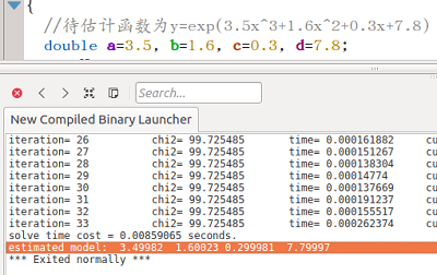
//待估计函数为y=exp(3.5x^3+1.6x^2+0.3x+7.8)
double a=3.5, b=1.6, c=0.3, d=7.8;
int N=100;
double w_sigma=1.0;
cv::RNG rng;
vector<double> x_data, y_data;
cout<<"generating data: "<<endl;
for (int i=0; i<N; i++)
{
double x = i/100.0;
x_data.push_back (x);
y_data.push_back (exp(a*x*x*x + b*x*x + c*x + d) + rng.gaussian (w_sigma));
cout<<x_data[i]<<"\t"<<y_data[i]<<endl;
}
//构建图优化,先设定g2o
//矩阵块:每个误差项优化变量维度为4,误差值维度为1
typedef g2o::BlockSolver<g2o::BlockSolverTraits<4,1>> Block;
// Step1 选择一个线性方程求解器
std::unique_ptr<Block::LinearSolverType> linearSolver (new g2o::LinearSolverDense<Block::PoseMatrixType>());
// Step2 选择一个稀疏矩阵块求解器
std::unique_ptr<Block> solver_ptr (new Block(std::move(linearSolver)));
// Step3 选择一个梯度下降方法,从GN、LM、DogLeg中选
g2o::OptimizationAlgorithmLevenberg* solver = new g2o::OptimizationAlgorithmLevenberg ( std::move(solver_ptr));
//g2o::OptimizationAlgorithmGaussNewton* solver = new g2o::OptimizationAlgorithmGaussNewton( std::move(solver_ptr));
//g2o::OptimizationAlgorithmDogleg* solver = new g2o::OptimizationAlgorithmDogleg(std::move(solver_ptr));
//稀疏优化模型
g2o::SparseOptimizer optimizer;
//设置求解器
optimizer.setAlgorithm(solver);
//打开调试输出
optimizer.setVerbose(true);
//往图中增加顶点
CurveFittingVertex* v = new CurveFittingVertex();
//这里的(0,0,0,0)可以理解为顶点的初值了,不同的初值会导致迭代次数不同,可以试试
v->setEstimate(Eigen::Vector4d(0,0,0,0));
v->setId(0);
optimizer.addVertex(v);
//往图中增加边
for (int i=0; i<N; i++)
{
//新建边带入观测数据
CurveFittingEdge* edge = new CurveFittingEdge(x_data[i]);
edge->setId(i);
//设置连接的顶点,注意使用方式
//这里第一个参数表示边连接的第几个节点(从0开始),第二个参数是该节点的指针
edge->setVertex(0, v);
//观测数值
edge->setMeasurement(y_data[i]);
//信息矩阵:协方差矩阵之逆,这里各边权重相同。这里Eigen的Matrix其实也是模板类
edge->setInformation(Eigen::Matrix<double,1,1>::Identity()*1/(w_sigma*w_sigma));
optimizer.addEdge(edge);
}
//执行优化
cout<<"start optimization"<<endl;
chrono::steady_clock::time_point t1 = chrono::steady_clock::now();//计时
//初始化优化器
optimizer.initializeOptimization();
//优化次数
optimizer.optimize(100);
chrono::steady_clock::time_point t2 = chrono::steady_clock::now();//结束计时
chrono::duration<double> time_used = chrono::duration_cast<chrono::duration<double>>( t2-t1 );
cout<<"solve time cost = "<<time_used.count()<<" seconds. "<<endl;
//输出优化值
Eigen::Vector4d abc_estimate = v->estimate();
cout<<"estimated model: "<<abc_estimate.transpose()<<endl;
return 0;
}
执行结果如下:
5.复杂一点的例子
前面的例子是利用g2o拟合曲线,但我们更想用它来优化位姿。下面的代码通过装载已知数据集的数据并对其进行优化。
//
// Created by root on 18-4-9.
//
#include "g2o/core/sparse_optimizer.h"
#include "g2o/core/block_solver.h"
#include "g2o/core/factory.h"
#include "g2o/core/optimization_algorithm_levenberg.h"
#include "g2o/solvers/cholmod/linear_solver_cholmod.h"
#include "g2o/types/slam2d/vertex_se2.h"
#include "g2o/types/slam3d/vertex_se3.h"
#include <iostream>
//G2O_USE_TYPE_GROUP保证能保证graph的load和save的成功
//也就是optimizer.load和optimizer.save在执行时有相对的类型对应.
//slam3d和slam2d对应不同的顶点和边的类型.这里都registration.
G2O_USE_TYPE_GROUP(slam3d);
G2O_USE_TYPE_GROUP(slam2d);
using namespace std;
using namespace g2o;
#define MAXITERATION 10
int main(){
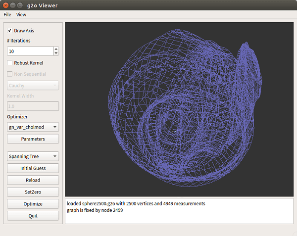
char* path = "sphere2500.g2o";
unique_ptr<BlockSolverX::LinearSolverType> linearSolver(new LinearSolverCholmod<BlockSolverX ::PoseMatrixType>());
unique_ptr<BlockSolverX> blockSolverX(new BlockSolverX(move(linearSolver)));
OptimizationAlgorithmLevenberg* solver = new OptimizationAlgorithmLevenberg(move(blockSolverX));
SparseOptimizer optimizer;
if(!optimizer.load(path)){
cout<<"Error loading file."<<endl;
return -1;
}else{
cout<<"Loaded "<<optimizer.vertices().size()<<" vertices"<<endl;
cout<<"Loaded "<<optimizer.edges().size()<<" edges."<<endl;
}
//这里这样做的目的是固定第一个点的位姿,当然不固定也可以,但最终优化的效果会有差别
//for sphere2500
VertexSE3* firstRobotPose = dynamic_cast<VertexSE3*>(optimizer.vertex(0));
//for manhattanOlson3500
//VertexSE2* firstRobotPose = dynamic_cast<VertexSE2*>(optimizer.vertex(0));
firstRobotPose->setFixed(true);
optimizer.setAlgorithm(solver);
optimizer.setVerbose(true);
cout<<"开始优化..."<<endl;
optimizer.initializeOptimization();
optimizer.optimize(MAXITERATION);
cout<<"优化完成..."<<endl;
optimizer.save("after.g2o");
optimizer.clear();
return 0;
}
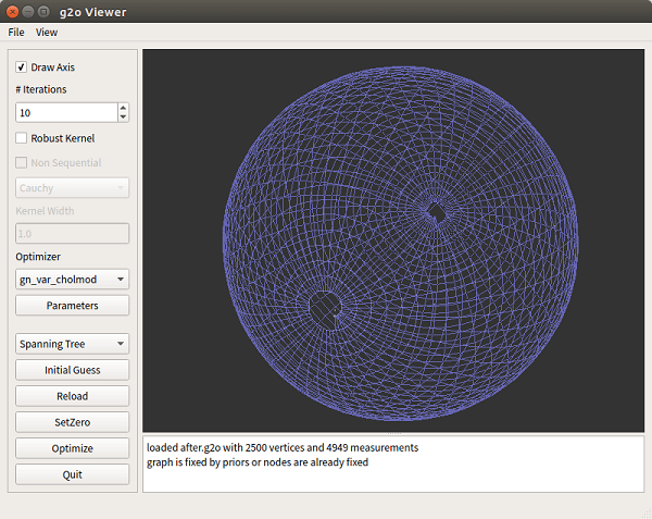
利用g2o viewer可以方便的对图进行可视化。首先是sphere2500.g2o,优化之前是这样的。
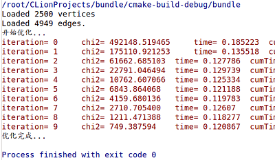
 优化完成后控制台输出如下
 优化后可视化的图如下
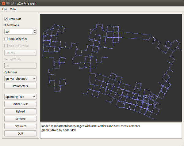
 同理,将上述代码稍作修改,对
manhattanOlson3500数据集优化。优化前图如下
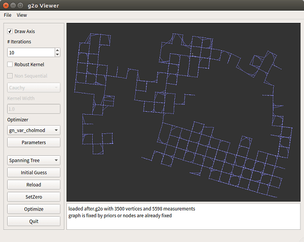
 优化后如下
优化后如下
 这段代码相对于曲线拟合反而要少一些,原因是这些顶点和边的类型在库中已经定义好了,不需要我们再重新去写了。
6.g2o库结构
在上面对g2o有了简单的了解以后,再看下面这张图会相对容易一些。
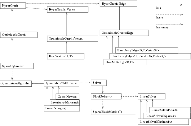 它表示了g2o中的类结构。
首先根据前面的代码经验可以发现,我们最终使用的
它表示了g2o中的类结构。
首先根据前面的代码经验可以发现,我们最终使用的optimizer是一个SparseOptimizer对象,因此我们要维护的就是它(对它进行各种操作)。
一个SparseOptimizer是一个可优化图(OptimizableGraph),也是一个超图(HyperGraph)。而图中有很多顶点(Vertex)和边(Edge)。顶点继承于BaseVertex,边继承于BaseUnaryEdge、BaseBinaryEdge或BaseMultiEdge。它们都是抽象的基类,实际有用的顶点和边都是它们的派生类。我们用SparseOptimizer.addVertex和SparseOptimizer.addEdge向一个图中添加顶点和边,最后调用SparseOptimizer.optimize完成优化。
在优化之前还需要制定求解器和迭代算法。一个SparseOptimizer拥有一个OptimizationAlgorithm,它继承自Gauss-Newton, Levernberg-Marquardt, Powell’s dogleg三者之一。同时,这个OptimizationAlgorithm拥有一个Solver,它含有两个部分。一个是 SparseBlockMatrix,用于计算稀疏的雅可比和海塞矩阵;一个是线性方程求解器,可从PCG、CSparse、Choldmod三选一,用于求解迭代过程中最关键的一步:
因此理清了g2o的结构,也就知道了其使用流程。在之前已经说过了,这里就再重复一遍。
- (1)选择一个线性方程求解器,PCG、CSparse、Choldmod三选一,来自
g2o/solvers文件夹 - (2)选择一个BlockSolver,用于求解雅克比和海塞矩阵,来自
g2o/core文件夹 - (3)选择一个迭代算法,GN、LM、DogLeg三选一,来自
g2o/core文件夹
7.双视图Bundle Adjustment(光束法平差)
如有两帧影像,我们的目标是估计相机在两帧影像间的运动。已知数据是相机内参(认为固定不变)和两张影像。 求解这个问题可以有两大类思路,一是通过特征点来求解,称为Sparse方式,特征点法。第二种是求解全部像素,称为Dense方式,直接法。 目前主流仍然在使用特征点法。所以这里就采用主流方法。
特征点方法的观点认为一个图像可以用几百个具有代表性的、比较稳定的点来表示。一旦有了这些点,就可以忽略图中的其余部分,而只关注这些点。(dense思路则反对这一观点,认为它丢弃了图像大部分信息,毕竟一个640x480的图有30万个点,而特征点只有几百个)。
在特征点的思路下,问题可以这样描述。有两张影像Img1、Img2,通过特征匹配共找到了N对同名点。
\[P_1=\left \{ p_1^1,p_1^2,...,p_1^N \right \},P_2=\left \{ p_2^1,p_2^2,...,p_2^N \right \}\]其中
\[p_1^i=\begin{pmatrix} u_1^i\\ v_1^i \end{pmatrix},p_2^i=\begin{pmatrix} u_2^i\\ v_2^i \end{pmatrix}\]已知相机内参矩阵为K,求解两张影像中相机的运动R,t。u、v为像素坐标。
假设某个特征点j在真实世界坐标系下的坐标为\(X^j\),在两幅影像的像素坐标系下分别为\(p_1^j,p_2^j\)。 我们要找的是真实坐标与像素坐标间的联系。 根据前面的知识可以知道,要想由真实坐标转到像素坐标,需要依次经过如下几步:
真实世界坐标->相机坐标->图像坐标->像素坐标
由相机坐标转像素坐标在这篇博客小孔成像模型里已经介绍了,这里直接给出公式
\[\begin{pmatrix} u\\ v\\ 1 \end{pmatrix}=\frac{1}{Z}K\begin{pmatrix} X\\ Y\\ Z \end{pmatrix}\]这里u、v为像素坐标,X、Y、Z为相机坐标系坐标。也就是说我们只需要再找到相机坐标与真实世界坐标间的变换矩阵T,既可以实现由真实坐标转像素坐标的流程了。而这个变换矩阵T其实就可以看成是相机此时的位姿或者说外方位元素。而这个很不巧,仅仅根据两张图片是无法获得相机的位姿的。但我们又必须要知道这个变换矩阵T来表示相机位姿,否则就没法继续算下去。所以没有办法,只能假设第一帧的这个变换矩阵T为单位阵。那么这样的话可以理解为真实世界坐标系与第一帧的相机坐标系重叠,也即真实世界坐标系下的坐标与第一帧相机坐标系下的坐标相等。
\[\begin{matrix} X_{camera} =T_{world}^{camera}X_{world}\\ T=I\\ X_{camera}=X_{world}\\ \end{matrix}\]所以,由上面的小孔成像模型则有
\[Z_1^j\begin{pmatrix} u_1^j\\ v_1^j\\ 1 \end{pmatrix}=K\begin{pmatrix} X_1^j\\ Y_1^j\\ Z_1^j \end{pmatrix}\]整理简写一下就是
\[Z_1^j\begin{pmatrix} p_1^j\\ 1 \end{pmatrix}=KX_1^j\]注意这里X不是单独的X变量,而是表示一个点坐标。同理,对于第二张影像我们也可以写出这个式子。
\[Z_2^j\begin{pmatrix} p_2^j\\ 1 \end{pmatrix}=KX_2^j\]而我们在之前假设,相机从图像1到2的运动为R,t。相机的运动其实可以看作是相机坐标系的运动,所以两个坐标系之间有下面的等式成立
\[X_2^j=RX_1^j+t\]将这个式子带入模型中去,有
\[Z_2^j\begin{pmatrix} p_2^j\\ 1 \end{pmatrix}=K(RX_1^j+t)\] \[Z_1^j\begin{pmatrix} p_1^j\\ 1 \end{pmatrix}=KX_1^j\]这个问题的传统做法是把两个方程中的\(X^j\)消去,得到只关于p、R、t的关系式,然后优化求解。这便是之前说的对极几何和基础矩阵(Essential Matrix)。理论上只需要大于等于8对同名点就能计算出R,t。当然尺度问题令说。
但在图优化中,我们可以这样写
\[\min_{X^j,R,t}(\begin{Vmatrix} \frac{1}{Z_1^j}K{X_1^j} - (p_1^j,1)^T \end{Vmatrix}^2+ \begin{Vmatrix} \frac{1}{Z_2^j}K\left({R{X_1^j} + t} \right) - (p_2^j,1)^T \end{Vmatrix}^2)\]由于各种噪声存在,投影关系不能完美满足,所以转而优化它们误差的二范数。因此对于每一个特征点都能写出一个二范数误差项。对它们求和,便得到了整个优化问题。
\[\min_{X,R,t}\sum_{j=1}^{N}(\begin{Vmatrix} \frac{1}{Z_1^j}K{X_1^j} - (p_1^j,1)^T \end{Vmatrix}^2+ \begin{Vmatrix} \frac{1}{Z_2^j}K\left({R{X_1^j} + t} \right) - (p_2^j,1)^T \end{Vmatrix}^2)\]这便是最小化重投影误差问题(Minimization of Reprojection Error)。它是一个非线性、非凸的优化问题。它的误差项是将像素坐标(观测到的投影位置)与3D点按照当前估计的位姿进行投影得到的位置相比较得到的误差,所以称为重投影误差。在实际操作中,通过调整每个\(X^j\),使得它们更符合每一次观测\(p^j\),使每个误差项都尽可能的小。
在这个双视图BA中,一共有两种节点:
- 相机位姿节点,表达相机所在位置,是一个SE(3)元素
- 特征点的空间位置节点,是一个XYZ坐标
边主要表示空间点到像素坐标的投影关系,也就是成像模型
\[Z^j\begin{pmatrix} p^j\\ 1 \end{pmatrix}=K(RX^j+t)\]代码实现
CMakeList
cmake_minimum_required(VERSION 3.10)
project(bundle)

set(CMAKE_CXX_STANDARD 11)

# 添加cmake模块以使用ceres库
list(APPEND CMAKE_MODULE_PATH ${PROJECT_SOURCE_DIR}/cmake_modules)

# 寻找G2O
include_directories(
        ${G2O_INCLUDE_DIRS}
        "/usr/include/eigen3"
        "/usr/include/suitesparse"
)

# OpenCV
find_package(OpenCV REQUIRED)
include_directories(${OpenCV_DIRS})

add_executable(bundle main.cpp ORBMatching.cpp ORBMatching.h sphere2500.cpp)

# 与G2O和OpenCV链接
target_link_libraries(bundle
        g2o_core g2o_stuff g2o_cli
        GL GLU cholmod
        g2o_incremental g2o_interactive g2o_interface g2o_parser
        g2o_solver_cholmod g2o_solver_csparse g2o_solver_dense g2o_solver_pcg
        g2o_types_icp g2o_types_sba g2o_types_sim3 g2o_types_slam2d g2o_types_slam3d
        ${OpenCV_LIBS}
        ${QT_LIBRARIES}
        ${QT_QTOPENGL_LIBRARY}
        ${GLUT_LIBRARY}
        ${OPENGL_LIBRARY}
        )
这里的list和上面第5部分的是一样的。尤其需要注意target link里面的各种库,Cholmod等等,如果少了可能编译会不通过。
C++代码
#include<iostream>
#include"ORBMatching.h"
#include<g2o/core/sparse_optimizer.h>
#include<g2o/core/block_solver.h>
#include<g2o/core/robust_kernel.h>
#include<g2o/core/robust_kernel_impl.h>
#include<g2o/core/optimization_algorithm_levenberg.h>
#include<g2o/solvers/cholmod/linear_solver_cholmod.h>
#include<g2o/types/slam3d/se3quat.h>
#include<g2o/types/sba/types_six_dof_expmap.h>
#include <chrono>

using namespace std;

void epipolar(vector<Point2f> pts1, vector<Point2f> pts2, double fx, double fy, double dx, double dy) {

    cout << "--------epipolar constraint--------" << endl;
    Point2d principal_point(dx, dy);
    Mat essential_matrix;
    double f = (fx + fy) / 2.0;
    essential_matrix = findEssentialMat(pts1, pts2, f, principal_point, RANSAC);
    Mat R, t;
    recoverPose(essential_matrix, pts1, pts2, R, t, f, principal_point);
    cout << "R:" << endl << R << endl;
    cout << "t:" << endl << t << endl;
    cout << "--------epipolar constraint--------" << endl;
    return;
}

void graph_optimization(vector<Point2f> &pts1, vector<Point2f> &pts2, double fx, double fy, double cx, double cy) {
    cout << "--------bundle adjustment--------" << endl;

    //矩阵块:每个误差项优化变量维度为6,误差值维度为3
    typedef g2o::BlockSolver<g2o::BlockSolverTraits<6, 3>> Block;
    // Step1 选择一个线性方程求解器
    std::unique_ptr<Block::LinearSolverType> linearSolver(new g2o::LinearSolverCholmod<Block::PoseMatrixType>());
    // Step2 选择一个稀疏矩阵块求解器
    std::unique_ptr<Block> solver_ptr(new Block(std::move(linearSolver)));
    // Step3 选择一个梯度下降方法,从GN、LM、DogLeg中选
    g2o::OptimizationAlgorithmLevenberg *solver = new g2o::OptimizationAlgorithmLevenberg(std::move(solver_ptr));

    g2o::SparseOptimizer optimizer;
    optimizer.setAlgorithm(solver);
    optimizer.setVerbose(true);

    //添加两个位姿节点,默认值为单位Pose,并且将第一个位姿节点也就是第一帧的位姿固定
    for (int i = 0; i < 2; i++) {
        g2o::VertexSE3Expmap *v = new g2o::VertexSE3Expmap();
        v->setId(i);
        if (i == 0) {
            v->setFixed(true);
        }
        v->setEstimate(g2o::SE3Quat());
        optimizer.addVertex(v);
    }

    //添加特征点作为节点
    for (size_t i = 0; i < pts1.size(); i++) {
        g2o::VertexSBAPointXYZ *v = new g2o::VertexSBAPointXYZ();
        v->setId(2 + i);
        //深度未知,设为1,利用相机模型,相当于是在求归一化相机坐标
        double z = 1;
        double x = (pts1[i].x - cx) * z / fx;
        double y = (pts1[i].y - cy) * z / fy;
        v->setMarginalized(true);
        v->setEstimate(Eigen::Vector3d(x, y, z));
        optimizer.addVertex(v);
    }

    //相机内参
    g2o::CameraParameters *camera = new g2o::CameraParameters(fx, Eigen::Vector2d(cx, cy), 0);
    camera->setId(0);
    optimizer.addParameter(camera);

    //添加第一帧中的边
    vector<g2o::EdgeProjectXYZ2UV *> edges;
    for (size_t i = 0; i < pts1.size(); i++) {
        g2o::EdgeProjectXYZ2UV *edge = new g2o::EdgeProjectXYZ2UV();

        edge->setVertex(0, dynamic_cast<g2o::VertexSBAPointXYZ *>(optimizer.vertex(i + 2)));
        edge->setVertex(1, dynamic_cast<g2o::VertexSE3Expmap *>(optimizer.vertex(0)));

        edge->setMeasurement(Eigen::Vector2d(pts1[i].x, pts1[i].y));
        edge->setInformation(Eigen::Matrix2d::Identity());
        edge->setParameterId(0, 0);
        edge->setRobustKernel(new g2o::RobustKernelHuber());

        optimizer.addEdge(edge);
        edges.push_back(edge);
    }

    //添加第二帧中的边
    for (size_t i = 0; i < pts2.size(); i++) {
        g2o::EdgeProjectXYZ2UV *edge = new g2o::EdgeProjectXYZ2UV();

        edge->setVertex(0, dynamic_cast<g2o::VertexSBAPointXYZ *>(optimizer.vertex(i + 2)));
        edge->setVertex(1, dynamic_cast<g2o::VertexSE3Expmap *>(optimizer.vertex(1)));

        edge->setMeasurement(Eigen::Vector2d(pts2[i].x, pts2[i].y));
        edge->setInformation(Eigen::Matrix2d::Identity());
        edge->setParameterId(0, 0);
        edge->setRobustKernel(new g2o::RobustKernelHuber());
        optimizer.addEdge(edge);
        edges.push_back(edge);
    }

    cout << "开始优化" << endl;
    chrono::steady_clock::time_point t1 = chrono::steady_clock::now();//计时
    optimizer.initializeOptimization();
    optimizer.optimize(10);
    chrono::steady_clock::time_point t2 = chrono::steady_clock::now();//结束计时
    cout << "优化完毕" << endl;

    chrono::duration<double> time_used = chrono::duration_cast<chrono::duration<double>>(t2 - t1);
    cout << "solve time cost = " << time_used.count() << " seconds. " << endl;

    //输出变换矩阵T
    g2o::VertexSE3Expmap *v = dynamic_cast<g2o::VertexSE3Expmap *>(optimizer.vertex(1));
    Eigen::Isometry3d pose = v->estimate();
    cout << "Pose=" << endl << pose.matrix() << endl;

    //优化后所有特征点的位置
    for (size_t i = 0; i < pts1.size(); i++) {
        g2o::VertexSBAPointXYZ *v = dynamic_cast<g2o::VertexSBAPointXYZ *>(optimizer.vertex(i + 2));
        cout << "vertex id:" << i + 2 << ",pos=";
        Eigen::Vector3d pos = v->estimate();
        cout << pos(0) << "," << pos(1) << "," << pos(2) << endl;
    }

    //估计inliner的个数
    int inliners = 0;
    for (auto e:edges) {
        e->computeError();
        //chi2()如果很大,说明此边的值与其它边很不相符
        if (e->chi2() > 1) {
            cout << "error = " << e->chi2() << endl;
        } else {
            inliners++;
        }
    }
    cout << "inliners in total points:" << inliners << "/" << pts1.size() + pts2.size() << endl;
    optimizer.save("ba.g2o");
    cout << "--------bundle adjustment--------" << endl;
    return;
};

double cx = 1535.89;
double cy = 2046.97;
double fx = 1536.2;
double fy = 1536.2;
string img_path1 = "/root/satellite_slam_data/tianjin/jpg2/VBZ1_201801051905_002_0002_L1A.jpg";
string img_path2 = "/root/satellite_slam_data/tianjin/jpg2/VBZ1_201801051905_002_0003_L1A.jpg";


int main(int argc, char **argv) {

    vector<Point2f> pts1, pts2;
    getMatchPoints(img_path1, img_path2, pts1, pts2);
    graph_optimization(pts1, pts2, fx, fy, cx, cy);
    epipolar(pts1, pts2, fx, fy, cx, cy);

    return 0;
}
代码中同时将利用对极约束求解位姿作为对比,同时运行了基于对极几何和基于Bundle Adjustment的求解,运行部分结果如下
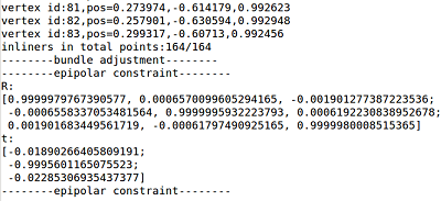 项目放在Github上了,点击查看。
8.参考资料
- https://blog.csdn.net/rs_huangzs/article/details/50574141
- https://blog.csdn.net/tian_123456789/article/details/51345189
- https://blog.csdn.net/qq_26849233/article/details/62218385
- https://blog.csdn.net/heyijia0327/article/details/47686523
本文作者原创,未经许可不得转载,谢谢配合